Part 5 Exploratory Analysis in R
For the exploratory analysis in R I focused on using the tm and quanteda (Benoit et al. 2021) packages: the former because of its simple methods for finding co-occurences and frequent terms across documents and the latter for its textstat sub-package and because it will also be the package I use for topic modeling in R.
With quanteda I created Document Term Matrixes from the corpus versions, which were then used for the majority of operations. This allowed me to look at frequency in a different way than I had done in Python where I was only using the corpus items.
library(tm)
raw_corpus<- VCorpus(DirSource("FILES/rbma-lectures-master/data_no_empty_files_new_file_names_no_intro")); r_corpus<- VCorpus(DirSource("FILES/RBMA_CLEAN_R_LEMM_V2")); py_corpus<- VCorpus(DirSource("FILES/RBMA_CLEAN_PY_LEMM_V2_POS"));
raw_dtm<- DocumentTermMatrix(raw_corpus); r_dtm<- DocumentTermMatrix(r_corpus); py_dtm<- DocumentTermMatrix(py_corpus)
A quick glance at the resulting DTMs show high percentages of sparsity so I decided to reduce their sizes to make them easier to handle and help me focus on the most useful and meaningful terms.
raw_dtm## <<DocumentTermMatrix (documents: 468, terms: 124509)>>
## Non-/sparse entries: 1018563/57251649
## Sparsity : 98%
## Maximal term length: 84
## Weighting : term frequency (tf)r_dtm## <<DocumentTermMatrix (documents: 468, terms: 44933)>>
## Non-/sparse entries: 518877/20509767
## Sparsity : 98%
## Maximal term length: 63
## Weighting : term frequency (tf)py_dtm## <<DocumentTermMatrix (documents: 468, terms: 37549)>>
## Non-/sparse entries: 531743/17041189
## Sparsity : 97%
## Maximal term length: 33
## Weighting : term frequency (tf)raw_dtm<- removeSparseTerms(raw_dtm, 0.5); r_dtm<- removeSparseTerms(r_dtm, 0.5); py_dtm<- removeSparseTerms(py_dtm, 0.5)
raw_dtm## <<DocumentTermMatrix (documents: 468, terms: 788)>>
## Non-/sparse entries: 278529/90255
## Sparsity : 24%
## Maximal term length: 11
## Weighting : term frequency (tf)r_dtm## <<DocumentTermMatrix (documents: 468, terms: 494)>>
## Non-/sparse entries: 172989/58203
## Sparsity : 25%
## Maximal term length: 12
## Weighting : term frequency (tf)py_dtm## <<DocumentTermMatrix (documents: 468, terms: 513)>>
## Non-/sparse entries: 180991/59093
## Sparsity : 25%
## Maximal term length: 12
## Weighting : term frequency (tf)5.1 Co-occurences
One the things I had struggled to easily do in Python was looking at co-occurences. However, this is much easier to do in R. The tm package provides the findAssocs method as a first step, which returns co-occurences within the DTM based on a specific term and correlation limit.
I decided to look at associations for ten words from the term frequency list produced in Python which I consider thematically important to the corpus. They are: “music”, “think”, “people”, “know”, “record”, “sound”, “time”, “song”, “listen” and “track.”
I set the correlation limit for each term to a level that would allow me to have enough results to analyze. In general that threshold was between 0.2 and 0.5 for the cleaned versions, and 0.3 to 0.5 for the raw corpus, denoting low to moderate levels of correlation.
To make analyzing the data easier I turned these results into a combined data frame. I first assigned the findAssocs searches to variables, then turned those variables into data frames containing columns for terms, score, and corpus source, and finally combined the data frames into one. I used the dplyr (Wickham et al. 2021) and qdap (Rinker 2020) packages to do this.
library(dplyr)
library (qdap)
#set associations to variables and turn into df
raw_music<- findAssocs(raw_dtm, "music", 0.3); raw_music<- list_vect2df(raw_music, col1 = "term", col2 = "association", col3 = "score"); r_music<- findAssocs(r_dtm, "music", 0.3); r_music<- list_vect2df(r_music, col1 = "term", col2 = "association", col3 = "score"); py_music<- findAssocs(py_dtm, "music", 0.3); py_music<- list_vect2df(py_music, col1 = "term", col2 = "association", col3 = "score")
music_assocs_df<- bind_rows(raw_music, r_music, py_music, .id = "corpus")
#think associations
raw_think<- findAssocs(raw_dtm, "think", 0.4); raw_think<- list_vect2df(raw_think, col1 = "term", col2 = "association", col3 = "score"); r_think<- findAssocs(r_dtm, "think", 0.4); r_think<- list_vect2df(r_think, col1 = "term", col2 = "association", col3 = "score"); py_think<- findAssocs(py_dtm, "think", 0.3); py_think<- list_vect2df(py_think, col1 = "term", col2 = "association", col3 = "score")
think_assocs_df<- bind_rows(raw_think, r_think, py_think, .id = "corpus")
#people association
raw_people<- findAssocs(raw_dtm, "people", 0.5); raw_people<- list_vect2df(raw_people, col1 = "term", col2 = "association", col3 = "score"); r_people<- findAssocs(r_dtm, "people", 0.4); r_people<- list_vect2df(r_people, col1 = "term", col2 = "association", col3 = "score"); py_people<- findAssocs(py_dtm, "people", 0.4); py_people<- list_vect2df(py_people, col1 = "term", col2 = "association", col3 = "score")
people_assocs_df<- bind_rows(raw_people, r_people, py_people, .id = "corpus")
#know association
raw_know<- findAssocs(raw_dtm, "know", 0.5); raw_know<- list_vect2df(raw_know, col1 = "term", col2 = "association", col3 = "score"); r_know<- findAssocs(r_dtm, "know", 0.5); r_know<- list_vect2df(r_know, col1 = "term", col2 = "association", col3 = "score"); py_know<- findAssocs(py_dtm, "know", 0.5); py_know<- list_vect2df(py_know, col1 = "term", col2 = "association", col3 = "score")
know_assocs_df<- bind_rows(raw_know, r_know, py_know, .id = "corpus")
#record association
raw_record<- findAssocs(raw_dtm, "record", 0.4); raw_record<- list_vect2df(raw_record, col1 = "term", col2 = "association", col3 = "score"); r_record<- findAssocs(r_dtm, "record", 0.4); r_record<- list_vect2df(r_record, col1 = "term", col2 = "association", col3 = "score"); py_record<- findAssocs(py_dtm, "record", 0.4); py_record<- list_vect2df(py_record, col1 = "term", col2 = "association", col3 = "score")
record_assocs_df<- bind_rows(raw_record, r_record, py_record, .id = "corpus")
#sound association
raw_sound<- findAssocs(raw_dtm, "sound", 0.3); raw_sound<- list_vect2df(raw_sound, col1 = "term", col2 = "association", col3 = "score"); r_sound<- findAssocs(r_dtm, "sound", 0.3); r_sound<- list_vect2df(r_sound, col1 = "term", col2 = "association", col3 = "score"); py_sound<- findAssocs(py_dtm, "sound", 0.3); py_sound<- list_vect2df(py_sound, col1 = "term", col2 = "association", col3 = "score")
sound_assocs_df<- bind_rows(raw_sound, r_sound, py_sound, .id = "corpus")
#time association
raw_time<- findAssocs(raw_dtm, "time", 0.5); raw_time<- list_vect2df(raw_time, col1 = "term", col2 = "association", col3 = "score"); r_time<- findAssocs(r_dtm, "time", 0.5); r_time<- list_vect2df(r_time, col1 = "term", col2 = "association", col3 = "score"); py_time<- findAssocs(py_dtm, "time", 0.5); py_time<- list_vect2df(py_time, col1 = "term", col2 = "association", col3 = "score")
time_assocs_df<- bind_rows(raw_time, r_time, py_time, .id = "corpus")
#song association
raw_song<- findAssocs(raw_dtm, "song", 0.4); raw_song<- list_vect2df(raw_song, col1 = "term", col2 = "association", col3 = "score"); r_song<- findAssocs(r_dtm, "song", 0.4); r_song<- list_vect2df(r_song, col1 = "term", col2 = "association", col3 = "score"); py_song<- findAssocs(py_dtm, "song", 0.4); py_song<- list_vect2df(py_song, col1 = "term", col2 = "association", col3 = "score")
song_assocs_df<- bind_rows(raw_song, r_song, py_song, .id = "corpus")
#listen association
raw_listen<- findAssocs(raw_dtm, "listen", 0.3); raw_listen<- list_vect2df(raw_listen, col1 = "term", col2 = "association", col3 = "score"); r_listen<- findAssocs(r_dtm, "listen", 0.3); r_listen<- list_vect2df(r_listen, col1 = "term", col2 = "association", col3 = "score"); py_listen<- findAssocs(py_dtm, "listen", 0.3); py_listen<- list_vect2df(py_listen, col1 = "term", col2 = "association", col3 = "score")
listen_assocs_df<- bind_rows(raw_listen, r_listen, py_listen, .id = "corpus")
#track association
raw_track<- findAssocs(raw_dtm, "track", 0.2); raw_track<- list_vect2df(raw_track, col1 = "term", col2 = "association", col3 = "score"); r_track<- findAssocs(r_dtm, "track", 0.2); r_track<- list_vect2df(r_track, col1 = "term", col2 = "association", col3 = "score"); py_track<- findAssocs(py_dtm, "track", 0.2); py_track<- list_vect2df(py_track, col1 = "term", col2 = "association", col3 = "score")
track_assocs_df<- bind_rows(raw_track, r_track, py_track, .id = "corpus")
assocs_df<- bind_rows(music_assocs_df, track_assocs_df, listen_assocs_df, song_assocs_df, time_assocs_df, sound_assocs_df, record_assocs_df, know_assocs_df, people_assocs_df, think_assocs_df)
DT::datatable(assocs_df)
Looking at these results, we see some expected combinations for the corpus’ central thematic term of “music”: “dance music,” “find music,” “world music,” “making/make music,” “interest(ing) music/interest(ed in) music,” “music culture,” “listen(ing to) music,” “music influence,” and “play music.”
Co-occurences for “record” and “sound” primarily reflect their usage as a noun or adjective rather than a verb: “make/buy/want (a) record,” “different sound,” “hit record,” “sound system,” “change (a/the) sound,” “sound effect,” “use sound,” “record(ing) studio.”
Both “think” and “people” returned some obvious results such as “people make/think” though the more interesting associations were with verbs such as “feel,” “want,” “try,” “see,” and “talk” which are all relevant to the creative process.
The results for “know,” “listen” and “time” were the least revealing and I’d argue these terms have more potential in the results for our other terms, such as “listen (to a) record/music.”
Lastly, “song” and “track” have a degree of interchangeability in everyday usage within music discourse and some of this is reflected in the results. “Take,” “put,” “hear,” “make,” “good,” “big,” “studio,” and “producer” appear as co-occurences for both terms. The differences between co-occurences for the two terms are equally interesting with “mix,” “dance,” and “vocal” appearing only with “track” while “beat,” “crazy,” and “love” appear only with “song.” In both cases some of these can feel a little counter-intuitive: one might expect “beat” to be more easily associated with “track” or “vocal” with “song.”
Seeing as these two terms appeared to have the most interplay, I decided to visualize their shared correlations in the cleaned versions via a plot, which shows “good”, “big”, and “start” as the co-occurences with the closest correlation threshold between both terms.17
corr1<- findAssocs(r_dtm, "song", 0.3)[[1]]; corr2<- findAssocs(r_dtm, "track", 0.2)[[1]]
corr1<- cbind(read.table(text = names(corr1), stringsAsFactors = FALSE), corr1); corr2 <- cbind(read.table(text = names(corr2), stringsAsFactors = FALSE), corr2)
library(dplyr)
#join and arrange the two correlation results
two_terms_corrs <- full_join(corr1, corr2)
library(tidyr)
two_terms_corrs_gathered <- gather(two_terms_corrs, term, correlation, corr1:corr2)
two_terms_corrs_gathered$term <- ifelse(two_terms_corrs_gathered$term  == "corr1", "song", "track")
#create a version with only joint correlations
two_terms_corrs_gathered_trim<- two_terms_corrs_gathered[c(58, 163, 61, 166, 21, 126, 22, 127, 31, 136, 16, 121, 47, 152, 32, 137, 13, 118, 14, 119, 57, 162),]
require(ggplot2)
ggplot(two_terms_corrs_gathered_trim, aes(x = V1, y = correlation, colour =  term ) ) +
  geom_point(size = 3) +
  xlab("Terms") +
  ylab(paste0("Correlation with the terms ", "\"", "song",  "\"", " and ",  "\"", "track", "\"")) +
  theme_bw() +
  theme(axis.text.x = element_text(angle = 90, hjust = 1, vjust = 0.5))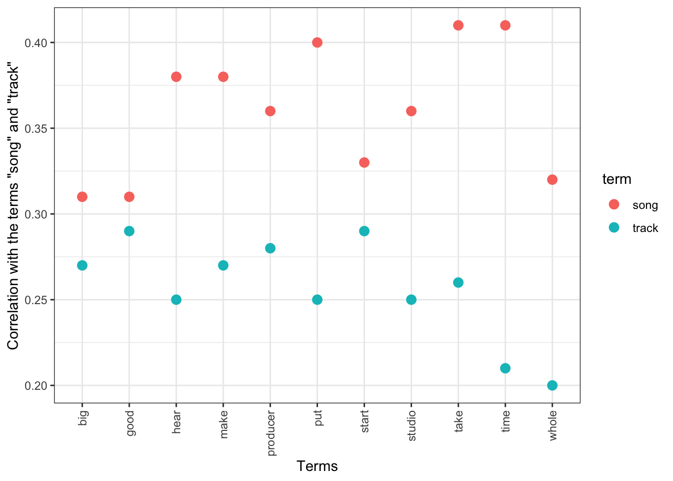
Next I used another tm method, findMostFreqTerms, which returns a list of lists of the most frequent terms for each document in the corpus. I set the limit to 5 and then bound these lists into a single data frame showing each list as a row for easy analysis. Below we can see the top 5 and bottom 5 results for the R version of the corpus.
n = 5
r_most_freq<- findMostFreqTerms(r_dtm, n = n)
r_most_freq<- do.call(rbind, lapply(r_most_freq, function(x) { x <- names(x);length(x)<-n;x }))
head(r_most_freq)
## [,1] [,2] [,3] [,4] [,5]
## a-guy-called-gerald.txt "actually" "call" "guy" "people" "time"
## addison-groove.txt "play" "make" "music" "track" "people"
## aisha-devi.txt "music" "actually" "voice" "will" "think"
## alec-empire.txt "people" "think" "music" "time" "maybe"
## alex-barck.txt "music" "record" "people" "think" "play"
## alex-rosner.txt "sound" "room" "good" "make" "put"tail(r_most_freq)## [,1] [,2] [,3] [,4] [,5]
## wu-tang-clan.txt "shit" "come" "time" "say" "right"
## xavier-veilhan.txt "work" "music" "art" "people" "time"
## yoshimio.txt "play" "right" "think" "record" "music"
## young-guru.txt "record" "people" "music" "make" "come"
## yury-chernavsky.txt "play" "music" "people" "yes" "first"
## yuzo-koshiro.txt "music" "time" "make" "video" "use"A look at these results shows many of the corpus’ most frequent terms I’ve already highlighted alongside some keywords that are more specific to each document: Yuzo Koshiro’s lecture features the term “video” no doubt in relation to his work in video games; the Wu-Tang Clan likes to swear and confirm each other’s statements; Xavier Veilhan, one of the few non-musicians in the corpus, talks about “art” rather than “music”; and renowned sound system engineer Alex Rosner focused his talk on the importance of sound to physical spaces which seems clearly represented by his top 5 most frequent terms.
n = 5
py_most_freq<- findMostFreqTerms(py_dtm, n = n)
py_most_freq<- do.call(rbind, lapply(py_most_freq, function(x) { x <- names(x);length(x)<-n;x }))
head(py_most_freq)
## [,1] [,2] [,3] [,4] [,5]
## a-guy-called-gerald.txt "like" "actually" "get" "would" "thing"
## addison-groove.txt "make" "music" "track" "like" "get"
## aisha-devi.txt "music" "actually" "like" "voice" "think"
## alec-empire.txt "like" "people" "think" "music" "stuff"
## alex-barck.txt "music" "like" "record" "people" "really"
## alex-rosner.txt "sound" "room" "get" "put" "make"tail(py_most_freq)## [,1] [,2] [,3] [,4] [,5]
## wu-tang-clan.txt "like" "get" "shit" "know" "come"
## xavier-veilhan.txt "work" "music" "like" "art" "thing"
## yoshimio.txt "like" "really" "play" "right" "record"
## young-guru.txt "like" "get" "thing" "record" "people"
## yury-chernavsky.txt "music" "like" "well" "people" "yes"
## yuzo-koshiro.txt "music" "game" "time" "like" "make"As expected the Python version has a little more noise from not having the custom stopwords removed though we can also see a similar pattern with one or two lecture-specific keyword popping up in the top 5.
5.2 Term Frequency vs Inverse Document Frequency
So far all the operations were conducted with DTMs created using term frequency as the weighting option, meaning that a word’s rank was based on its frequency across all documents: every time the word appears it gets a count and thus increases in rank. However, term frequency does not equate relevance as shown by the most frequent list of the raw corpus in 4.3. While term frequency is clearly useful to bring the main themes of a corpus to the fore as we’ve seen it does not necessarily tell us anything about their importance. I know music is central to this corpus, but I also know that music is a broad umbrella and that different types of musicians and practices are represented in the corpus.
To try and get at this I decided to look at the DTMs using the Inverse Document Frequency approach (tf-idf) whereby words are weighted based on term frequency as well as relative importance to a document. The expectation then is that the results will now show lists of terms that are more specific to each documents as well as bring forward sub-themes across the corpus rather than the overall themes we’ve already seen.
First I set the DTMs to variables and sparsed them as I’d done with the term frequency versions.
raw_dtm_idf<- DocumentTermMatrix(raw_corpus, control = list(weighting = weightTfIdf)); r_dtm_idf<- DocumentTermMatrix(r_corpus, control = list(weighting = weightTfIdf)); py_dtm_idf<- DocumentTermMatrix(py_corpus, control = list(weighting = weightTfIdf))
raw_dtm_idf<- removeSparseTerms(raw_dtm_idf, 0.5); r_dtm_idf<- removeSparseTerms(r_dtm_idf, 0.5); py_dtm_idf<- removeSparseTerms(py_dtm_idf, 0.5)
raw_dtm_idf
## <<DocumentTermMatrix (documents: 468, terms: 750)>>
## Non-/sparse entries: 260745/90255
## Sparsity : 26%
## Maximal term length: 11
## Weighting : term frequency - inverse document frequency (normalized) (tf-idf)r_dtm_idf## <<DocumentTermMatrix (documents: 468, terms: 482)>>
## Non-/sparse entries: 167373/58203
## Sparsity : 26%
## Maximal term length: 12
## Weighting : term frequency - inverse document frequency (normalized) (tf-idf)py_dtm_idf## <<DocumentTermMatrix (documents: 468, terms: 493)>>
## Non-/sparse entries: 171631/59093
## Sparsity : 26%
## Maximal term length: 12
## Weighting : term frequency - inverse document frequency (normalized) (tf-idf)Next I look at the top terms in each new DTM.
raw_idf_head<- head(data.frame(sort(colSums(as.matrix(raw_dtm_idf)), decreasing=TRUE)), 10); colnames(raw_idf_head)[1]<- "frequency"
r_idf_head<- head(data.frame(sort(colSums(as.matrix(r_dtm_idf)), decreasing=TRUE)), 10); colnames(r_idf_head)[1]<- "frequency"
py_idf_head<- head(data.frame(sort(colSums(as.matrix(py_dtm_idf)), decreasing=TRUE)), 10); colnames(py_idf_head)[1]<- "frequency"
raw_idf_head
## frequency
## gonna 0.1709571
## hip-hop 0.1502452
## black 0.1406327
## she 0.1355853
## jazz 0.1327173
## drum 0.1318957
## electronic 0.1309645
## yeah. 0.1299675
## song 0.1274526
## [laughs] 0.1249164r_idf_head## frequency
## shit 0.4548952
## hiphop 0.3880062
## remix 0.3873030
## band 0.3457131
## master 0.3359250
## song 0.3236251
## london 0.3177508
## tune 0.3163744
## sing 0.3117608
## video 0.3096802py_idf_head ## frequency
## shit 0.3948568
## gonna 0.3287453
## band 0.3141501
## hip 0.3060792
## master 0.2910337
## tune 0.2798423
## jazz 0.2793999
## laughter 0.2784546
## london 0.2778346
## video 0.2733863As expected we can now see a different set of terms, with some of the sub-themes I’d hoped to see: “hip-hop,” “jazz,” and “electronic” are potentially important genres, which I know to be the case based on my knowledge of the corpus and something that could be worth investigating further by adding metadata information to the documents about the primary genres each lecture features; “remix” and “master” are two creative practices that show up likely due to the fact there is at least one lecture with a mastering engineer every year and because both remixes and mastering are part and parcel of how many DJs and producers work; “song,” and its alternative “tune” (in the Python version), is the only term to still appear from the ten I’d selected as central to the themes based on the most common words; “shit” appears to be the preferred swear word; and “London” might be an important city to our corpus.
Next I looked at the most frequent terms for each document again, comparing tf and tf-idf. The tf version of the raw corpus tells us nothing meaningful, as expected, however the tf-idf version helps cut through some of the noise to bring themes for each document to the fore. Overall the results for the raw version remain noisy.
n = 5
raw_most_freq_idf<- findMostFreqTerms(raw_dtm_idf, n = n)
raw_most_freq_idf<- do.call(rbind, lapply(raw_most_freq_idf, function(x) { x <- names(x);length(x)<-n;x }))
raw_most_freq<- findMostFreqTerms(raw_dtm, n = n)
raw_most_freq<- do.call(rbind, lapply(raw_most_freq, function(x) { x <- names(x);length(x)<-n;x }))
head(raw_most_freq_idf)
## [,1] [,2] [,3] [,4] [,5]
## a-guy-called-gerald.txt "anyway," "guy" "basically," "basically" "you’d"
## addison-groove.txt "gonna" "drum" "track" "track." "track,"
## aisha-devi.txt "voice" "space" "pop" "produce" "course"
## alec-empire.txt "“ok," "go," "example," "felt" "“this"
## alex-barck.txt "jazz" "hip-hop" "less" "label" "label,"
## alex-rosner.txt "bass" "room" "high" "eight" "middle"tail(raw_most_freq_idf)## [,1] [,2] [,3] [,4] [,5]
## wu-tang-clan.txt "gonna" "felt" "style" "like," "lost"
## xavier-veilhan.txt "art" "she" "interested" "rather" "her"
## yoshimio.txt "free" "recording" "drums" "right?" "applause)"
## young-guru.txt "gonna" "hip-hop" "young" "york" "“ok,"
## yury-chernavsky.txt "created" "jazz" "sing" "yes," "such"
## yuzo-koshiro.txt "space" "create" "created" "so," "released"The differences between tf and tf-idf become much clearer with the cleaned versions.
r_most_freq_idf<- findMostFreqTerms(r_dtm_idf, n = n)
r_most_freq_idf<- do.call(rbind, lapply(r_most_freq_idf, function(x) { x <- names(x);length(x)<-n;x }))
head(r_most_freq_idf)
## [,1] [,2] [,3] [,4] [,5]
## a-guy-called-gerald.txt "machine" "basically" "anyway" "state" "push"
## addison-groove.txt "drum" "exist" "london" "machine" "track"
## aisha-devi.txt "voice" "space" "sing" "pop" "connect"
## alec-empire.txt "video" "hey" "weird" "american" "boy"
## alex-barck.txt "tune" "jazz" "hiphop" "remix" "sample"
## alex-rosner.txt "system" "room" "ear" "level" "bass"tail(r_most_freq_idf)## [,1] [,2] [,3] [,4] [,5]
## wu-tang-clan.txt "shit" "brother" "street" "family" "respect"
## xavier-veilhan.txt "art" "relationship" "form" "choose" "rather"
## yoshimio.txt "vocal" "free" "sing" "drum" "instrument"
## young-guru.txt "engineer" "hiphop" "york" "session" "genre"
## yury-chernavsky.txt "jazz" "sing" "boy" "musician" "country"
## yuzo-koshiro.txt "video" "program" "company" "street" "create"We can now see the importance of machines to lectures by A Guy Called Gerald and Addison Groove, two artists who have made drum machines and synthesizers a key part of their practice. Aïsha Devi has “voice”, “space”, and “sing” in her top 5, which are all key aspects of her practice. It becomes clearer that Alex Barck is a DJ with a penchant for jazz, hip-hop, and remixes. The Wu still swears a lot but we can also now see the importance of familial bonds and earning respect to their career. “Form” now appears in Veilhan’s top 5 alongside “art,” a refining of his position as a sculptor in a corpus full of musicians. Yoshimio’s varied career is captured in the prominence of “free” alongside instruments she plays and uses. And Young Guru and Yuri Chernavsky are now more clearly defined: the former as a hip-hop engineer and the latter as a jazz musician.
Similar results can be seen in the Python version, though again the presence of the custom stopwords removed from R create additional noise.
py_most_freq_idf<- findMostFreqTerms(py_dtm_idf, n = n)
py_most_freq_idf<- do.call(rbind, lapply(py_most_freq_idf, function(x) { x <- names(x);length(x)<-n;x }))
head(py_most_freq_idf)
## [,1] [,2] [,3] [,4] [,5]
## a-guy-called-gerald.txt "machine" "basically" "anyway" "state" "push"
## addison-groove.txt "gonna" "noise" "drum" "london" "exist"
## aisha-devi.txt "voice" "space" "sing" "electronic" "pop"
## alec-empire.txt "noise" "video" "felt" "hey" "game"
## alex-barck.txt "tune" "jazz" "hip" "sample" "less"
## alex-rosner.txt "low" "system" "room" "ear" "red"tail(py_most_freq_idf)## [,1] [,2] [,3] [,4] [,5]
## wu-tang-clan.txt "shit" "brother" "gonna" "game" "street"
## xavier-veilhan.txt "art" "relationship" "form" "rather" "musician"
## yoshimio.txt "vocal" "free" "sing" "drum" "instrument"
## young-guru.txt "gonna" "hip" "hop" "york" "session"
## yury-chernavsky.txt "jazz" "sing" "boy" "musician" "country"
## yuzo-koshiro.txt "game" "video" "program" "company" "street"5.3 Collocations
Collocations are another type of semantic linking between words that is easier to explore in R, allowing me to look a little beyond co-occurences. To do this I used the textstat sub-package within quanteda, first setting up new corpus objects using quanteda.
library(quanteda)
raw_corpus_q<- corpus(raw_corpus); r_corpus_q<- corpus(r_corpus); py_corpus_q<- corpus(py_corpus)
docnames(raw_corpus_q)<- docvars(raw_corpus_q, "id"); docnames(r_corpus_q)<- docvars(r_corpus_q, "id"); docnames(py_corpus_q)<- docvars(py_corpus_q, "id")
I first looked for bigrams, combinations of two words, in the cleaned versions as the raw version doesn’t tell us anything meaningful.
library(quanteda.textstats)
r_col<- textstat_collocations(r_corpus_q, size = 2, min_count = 500)
r_col<- r_col[order(r_col$count, decreasing = TRUE)]
DT::datatable(r_col)py_col<- textstat_collocations(py_corpus_q, size = 2, min_count = 500)
py_col<- py_col[order(py_col$count, decreasing = TRUE)]
DT::datatable(py_col)Just as “London” had popped up in the top 10 terms of the tf-idf versions, here we see “New York” as another potentially important location. Both of these results lead me to think that it would be interesting to use Named Entities and network analysis on locations to see what patterns might emerge.
“Hip hop” shows up again (but not in the R version as the removal of the punctation turned it into one word as we can see in the tf-idf version of the DTM), as do “electronic music” and “dance music” further hinting that these are key genres/sub-themes within the overall music theme. We also see similarities with the co-occurences we analyzed above and which are more emblematic of the corpus’ overall theme: “make music/record,” “play music,” “drum machine,” “record label.”
Next I looked for trigrams, three word combinations, lowering the count threshold to 50.
r_col_3<- textstat_collocations(r_corpus_q, size = 3, min_count = 50)
r_col_3<- r_col_3[order(r_col_3$count, decreasing = TRUE)]
DT::datatable(r_col_3)py_col_3<- textstat_collocations(py_corpus_q, size = 3, min_count = 50)
py_col_3<- py_col_3[order(py_col_3$count, decreasing = TRUE)]
DT::datatable(py_col_3)Overall trigrams are most revealing of the way interviews in this corpus are conducted: “talk (a) little bit” (which became bite in the lemmatizing process), “tell us (a) little,” “play (a) little bit” are all recurring prompts from hosts while “blah blah blah” and “yeah yeah yeah” are often used by both lecturers and hosts to simplify stories.
One last thing to note is the appearance of various artist names such (A) Guy Called Gerald, (A) Tribe Called Quest, Herb Power Jr, Mario Caldato Jr, De La Soul, and Mike Will Made-It (shown as Mike Will Make) whose tri- and quadgram names are ideal targets for the collocations.
References
Code for the plot function is adapted from the following thread: https://stackoverflow.com/questions/36326056/r-visualize-correlated-words-against-one-or-more-words)↩︎